ACS microdata
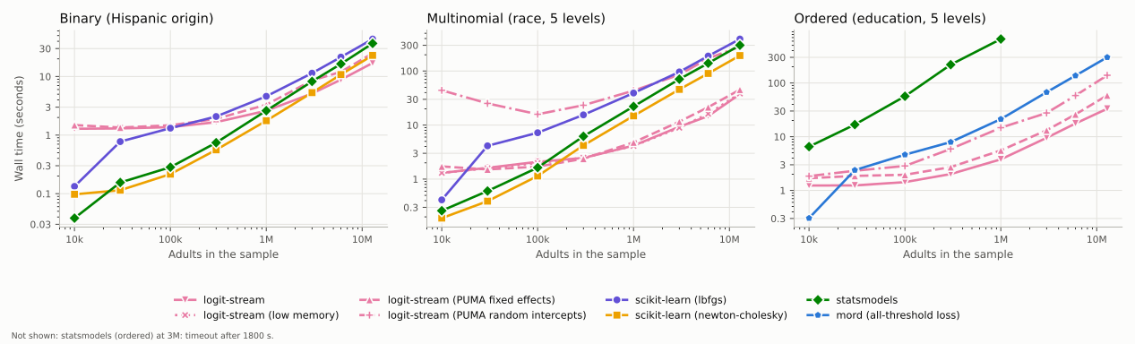
Three models of a demographic imputation, fitted to the adults of the American Community Survey 2019–2023 5-year Public Use Microdata Sample, from a random 10,000 of them to all 12,853,377:
model |
outcome |
coefficients |
|---|---|---|
binary |
Hispanic or Latino origin (13.5%) |
41 |
multinomial |
race and ethnicity in five groups: White (base), Black, Hispanic, Asian or Pacific Islander, other (incl. American Indian, multiracial) |
164 |
ordered |
educational attainment in five levels, adults 25 and over |
40 + 4 cutpoints |
on the same covariates: age group (7) and its interaction with sex,
personal income group (7, in 2023 dollars), citizenship and nativity (4),
English ability (4), marital status (5), disability, and Census division (9).
benchmarks/prepare_acs.py builds the data from the Census Bureau’s files;
the rows are in a random order, so the first n are a random sample of n.
Two notes on the specification. The division, not the state, is the
geography, and two rare categories are merged (the territory-born with the
US-born, “not well” with “not at all” for English): at 10,000 rows, states and
rare categories leave some cells without anyone of some race, which separates
their coefficients – their maximum-likelihood estimates are infinite – and
turns the comparison into one of how each library fails. And logit-stream is
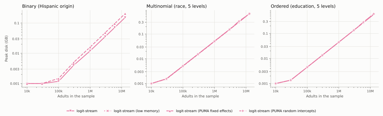
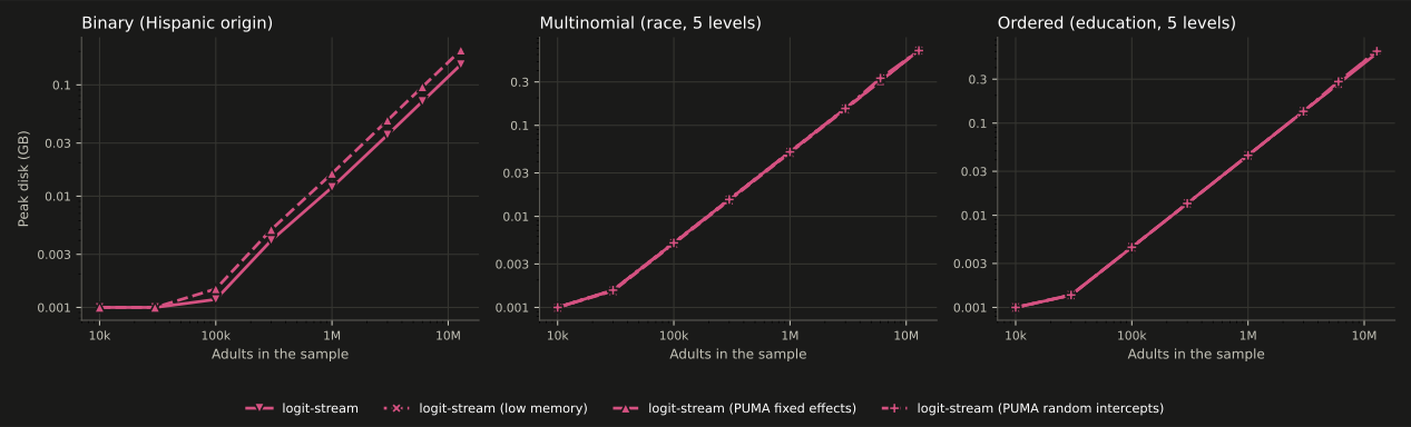
also run with the 2,462 PUMAs absorbed as a fixed effect in place of the
divisions (dashed in the figures): a richer model, which the in-memory
libraries could fit only with 2,461 indicator columns per equation. And it is
run with random PUMA intercepts in their place (dash-dotted;
experimental, see random intercepts): the
same richer model with the PUMA effects drawn from a normal distribution
whose covariance across the outcome levels is estimated, by Laplace’s
approximation (the default; the tables also have it within fixed state
effects). On all 12.9 million adults it took 283 s for the multinomial and
139 s for the ordered logit, 6.3 and 2.4 times the fixed-effect fits, with
about the same memory: each read also gathers the approximation’s
third-derivative terms, 64 per PUMA for the multinomial’s four equations.
The joint-mode approximation (random_method="joint-mode") is cheaper but
less exact: on all 12.9 million adults, with ~5,000 adults per PUMA, its
multinomial coefficients were up to 0.41 standard errors from Laplace’s (the
ordered logit’s, 0.06; the standard deviations agreed to 0.3%). The small
samples are the slow ones for the multinomial: at 10,000 adults a PUMA has about
four, so the effects’ covariance is weakly determined and its updates converge
slowly (44 s, 204 iterations; see the design notes).
The multinomial logit is also fitted with the discrete-choice libraries
xlogit and jaxlogit, which take long-format data: one row per person and
outcome level. xlogit is given the 40 covariates as individual-specific
variables (isvars) and expands them per level itself. jaxlogit has no
individual-specific variables, so the benchmark expands the design for it,
164 columns per row, the same array xlogit builds internally; the
expansion is timed with the reading. jaxlogit fits mixed logit only, and
runs here with no random parameters, which is this model. xlogit runs with
standard errors from the outer product of the gradients (num_hess=False):
its default numerical Hessian makes K(K+1) = 27,060 passes over the data
for these 164 coefficients.
Where the libraries finished, their coefficients agree with logit-stream’s to
within 1e-5 (scikit-learn’s L-BFGS, which stops on its own gradient
tolerance), 1e-7 (its Newton–Cholesky) and 1e-8 (statsmodels’ Newton). The R
libraries agree to within 5e-9 (glm, fixest), 2e-10 (clm) and 5e-5 (polr);
nnet’s multinom, whose BFGS stops at a relative tolerance of 1e-8, to within
1e-3. For
the ordered logit, statsmodels’ OrderedModel agrees to within 4e-4: its
default optimizer, BFGS, stops before Newton’s method would. mord’s
LogisticAT differs by 0.02 to 0.06 at every size. That isn’t a convergence
failure: mord minimizes a different loss, the “all-threshold” surrogate of
Rennie and Srebro (2005), not the ordered-logit likelihood, so it estimates a
different model with the same parameters. It’s included because it’s the
scikit-learn-style ordinal regression people use. The ordered logit’s main
effect of sex is not compared: in the 25-and-over sample the formula’s
reference age group (18–24) is absent, so logit-stream’s reference is a
different age group from the other libraries’; the fits are the same. The
numbers are in
benchmarks/results/acs.csv.
Results
All 12,853,377 adults, the largest fit of each model (the tables have every size):
model |
logit-stream |
fastest alternative |
|---|---|---|
binary, 41 coefficients |
17 s, 2.7 GB |
23 s, 12.0 GB (scikit-learn, Newton–Cholesky) |
multinomial, 164 coefficients |
37 s, 1.3 GB |
194 s, 13.3 GB (scikit-learn, Newton–Cholesky) |
ordered, 40 + 4 coefficients |
33 s, 1.2 GB |
301 s, 8.2 GB (mord, a different loss); R’s clm and polr ran out of memory |
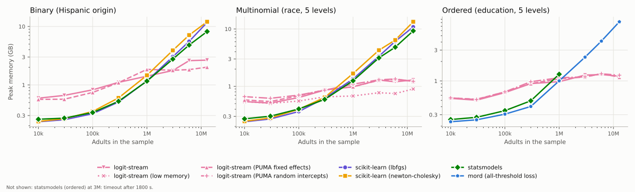
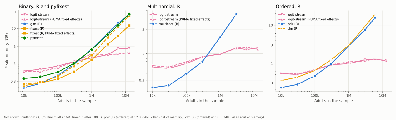
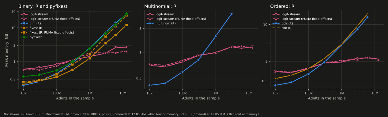
Memory is flat in the multinomial and ordered logit. logit-stream held 1.0 to 1.3 GB from 1 million to 12.9 million adults; the in-memory libraries grow in proportion to the data, to 8–13 GB.
The binary logit has the least to gain, since scikit-learn’s Newton–Cholesky solver takes the same six Newton steps in memory. It is faster below about 3 million adults (1.8 s against 2.6 s at 1 million), and logit-stream from there (5.1 s against 5.3 s at 3 million, 17 s against 23 s at 12.9 million), with about a quarter of the memory. (The plain binary logit runs through a fused, parallel kernel in hdfe-stream 0.6; before it, 40 s at 12.9 million adults.)
The multinomial and ordered logit are faster than every in-memory library from about 300,000 adults (the ordered, from 30,000), and at 12.9 million adults the multinomial took 5 times less than scikit-learn’s Newton–Cholesky and 8 times less than statsmodels’. statsmodels’
OrderedModeltook 11 minutes at a million adults and timed out at 3 million.Fixed effects for the 2,462 PUMAs cost 1.2 to 1.8 times the plain fit (binary 25 s, multinomial 45 s, ordered 59 s at 12.9 million adults); random intercepts, 283 s (multinomial) and 139 s (ordered).
Small samples: a fit costs about 1.3 s whatever the size, mostly fixed overhead, and scikit-learn’s and statsmodels’ finish in under a second at 10,000 adults.
On a GPU, the multinomial and ordered fits of all 12.9 million adults took 6.5 s and 5.4 s: see GPU.
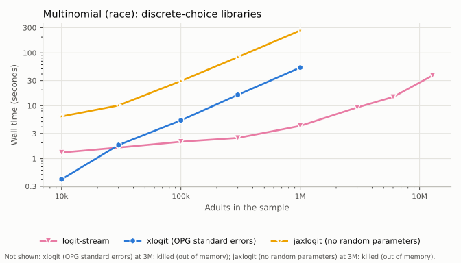
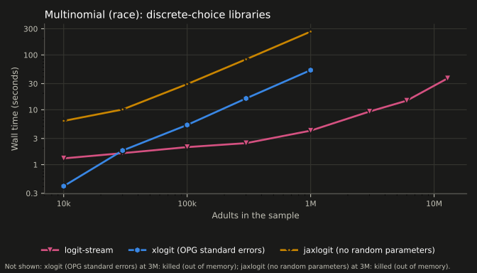
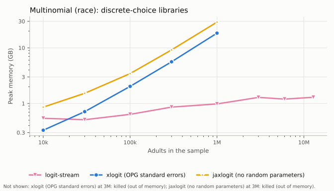
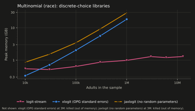
The discrete-choice libraries on the multinomial logit are in their own figure, so that every color in a figure can be told from every other. Long-format data cost them one row per person and level, and the expanded design 164 columns per row: at a million adults xlogit took 53 s and 18.4 GB and jaxlogit 267 s and 29.0 GB (nearly all of this machine’s memory), against logit-stream’s 4.2 s and 1.0 GB, and both ran out of memory at 3 million. At 10,000 adults xlogit is faster (0.4 s against 1.3 s). xlogit agrees with logit-stream to within 1e-5; jaxlogit to within 3e-4, its L-BFGS stopping on its own gradient tolerance after 135 to 165 iterations.
R and pyfixest
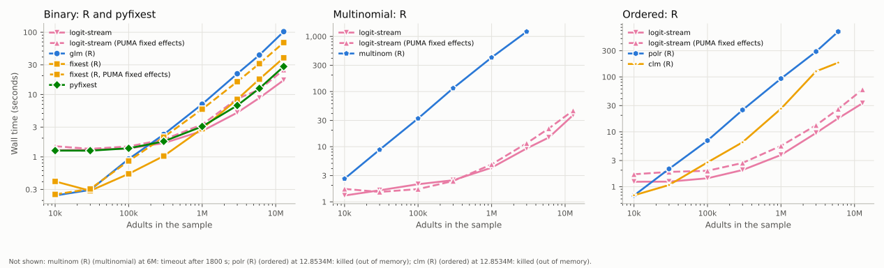
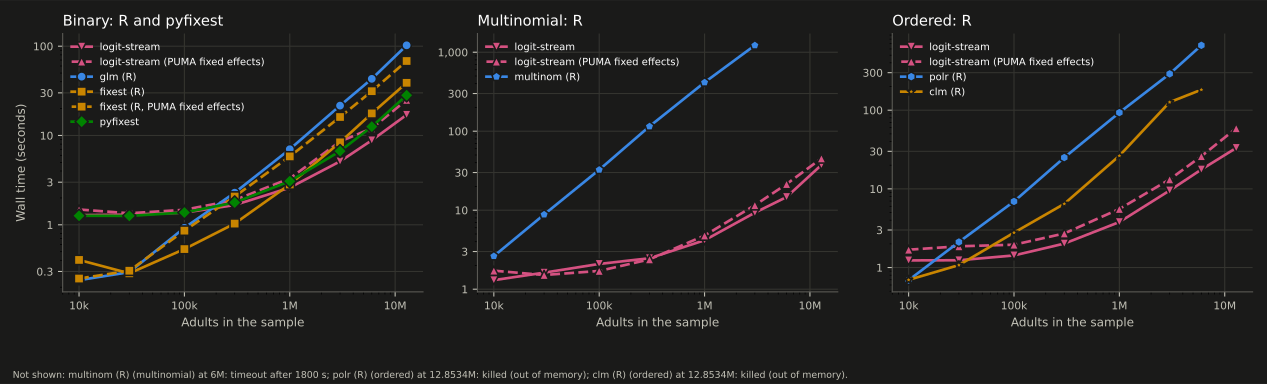
R’s glm, fixest (given every CPU, as in hdfe-stream’s benchmarks) and
pyfixest fit the binary logit, with fixest and logit-stream also with the
PUMA fixed effects; nnet::multinom fits the multinomial logit and MASS::polr
and ordinal::clm the ordered logit. At 12.9 million adults logit-stream’s
binary logit took 17 s and 2.7 GB, against 28 s and 26 GB for pyfixest,
39 s and 12 GB for fixest and 102 s and 25 GB for glm. multinom took 20
minutes at 3 million adults (logit-stream, 9 s) and timed out at 6 million.
polr took 5 and 11 minutes at 3 and 6 million adults and clm 2 and 3
(clm reported that it had not converged at both sizes, though its estimates
agree with logit-stream’s to 4e-11), and both ran out of memory at 12.9 million (this machine has 30 GB). The
R packages other than fixest ran with one thread.
Tables
The numbers behind the figures. A dash means the configuration was not run at that size, because it failed or timed out at a smaller one.
Binary logit
Wall time (seconds)
n |
logit-stream |
logit-stream (PUMA fixed effects) |
scikit-learn (lbfgs) |
scikit-learn (newton-cholesky) |
statsmodels |
|---|---|---|---|---|---|
10,000 |
1.3 |
1.5 |
0.13 |
0.10 |
0.04 |
30,000 |
1.3 |
1.3 |
0.77 |
0.11 |
0.16 |
100,000 |
1.4 |
1.5 |
1.3 |
0.22 |
0.28 |
300,000 |
1.7 |
1.9 |
2.1 |
0.56 |
0.74 |
1,000,000 |
2.6 |
3.3 |
4.6 |
1.8 |
2.6 |
3,000,000 |
5.1 |
8.6 |
11.4 |
5.3 |
8.2 |
6,000,000 |
8.8 |
12.0 |
21.5 |
10.8 |
16.4 |
12,853,377 |
17.1 |
25.0 |
43.7 |
23.0 |
36.8 |
Peak memory (GB)
n |
logit-stream |
logit-stream (PUMA fixed effects) |
scikit-learn (lbfgs) |
scikit-learn (newton-cholesky) |
statsmodels |
|---|---|---|---|---|---|
10,000 |
0.59 |
0.57 |
0.23 |
0.24 |
0.26 |
30,000 |
0.66 |
0.57 |
0.25 |
0.26 |
0.27 |
100,000 |
0.83 |
0.74 |
0.32 |
0.35 |
0.34 |
300,000 |
1.11 |
1.09 |
0.51 |
0.60 |
0.53 |
1,000,000 |
1.42 |
1.85 |
1.17 |
1.46 |
1.16 |
3,000,000 |
1.77 |
1.78 |
3.04 |
3.90 |
2.77 |
6,000,000 |
2.61 |
1.83 |
5.56 |
7.12 |
4.82 |
12,853,377 |
2.66 |
2.02 |
11.72 |
12.03 |
8.20 |
Multinomial logit
Wall time (seconds)
n |
logit-stream |
logit-stream (low memory) |
logit-stream (PUMA fixed effects) |
logit-stream (PUMA random intercepts) |
logit-stream (state fixed + PUMA random) |
scikit-learn (lbfgs) |
scikit-learn (newton-cholesky) |
statsmodels |
xlogit (OPG standard errors) |
jaxlogit (no random parameters) |
|---|---|---|---|---|---|---|---|---|---|---|
10,000 |
1.3 |
1.3 |
1.7 |
44.0 |
54.3 |
0.41 |
0.19 |
0.26 |
0.41 |
6.3 |
30,000 |
1.6 |
1.6 |
1.5 |
25.2 |
27.0 |
4.1 |
0.39 |
0.60 |
1.8 |
10.1 |
100,000 |
2.1 |
2.0 |
1.7 |
15.9 |
18.5 |
7.2 |
1.1 |
1.6 |
5.3 |
29.4 |
300,000 |
2.5 |
2.5 |
2.4 |
23.3 |
27.0 |
15.4 |
4.2 |
6.2 |
16.1 |
83.4 |
1,000,000 |
4.2 |
4.1 |
4.8 |
43.4 |
50.2 |
39.2 |
14.8 |
22.1 |
52.9 |
267 |
3,000,000 |
9.3 |
8.9 |
11.6 |
85.5 |
87.1 |
96.3 |
45.7 |
70.7 |
out of memory |
out of memory |
6,000,000 |
14.7 |
16.2 |
21.4 |
172 |
169 |
189 |
90.3 |
140 |
– |
– |
12,853,377 |
37.4 |
38.3 |
45.2 |
283 |
318 |
391 |
194 |
301 |
– |
– |
Peak memory (GB)
n |
logit-stream |
logit-stream (low memory) |
logit-stream (PUMA fixed effects) |
logit-stream (PUMA random intercepts) |
logit-stream (state fixed + PUMA random) |
scikit-learn (lbfgs) |
scikit-learn (newton-cholesky) |
statsmodels |
xlogit (OPG standard errors) |
jaxlogit (no random parameters) |
|---|---|---|---|---|---|---|---|---|---|---|
10,000 |
0.54 |
0.54 |
0.58 |
0.66 |
0.67 |
0.24 |
0.25 |
0.27 |
0.33 |
0.86 |
30,000 |
0.51 |
0.51 |
0.54 |
0.62 |
0.63 |
0.27 |
0.28 |
0.30 |
0.71 |
1.53 |
100,000 |
0.64 |
0.55 |
0.69 |
0.70 |
0.71 |
0.36 |
0.40 |
0.40 |
2.03 |
3.45 |
300,000 |
0.86 |
0.66 |
0.87 |
0.86 |
0.92 |
0.62 |
0.64 |
0.59 |
5.62 |
9.19 |
1,000,000 |
0.98 |
0.68 |
0.98 |
1.09 |
0.96 |
1.35 |
1.67 |
1.25 |
18.38 |
29.04 |
3,000,000 |
1.29 |
0.77 |
1.28 |
1.30 |
1.33 |
3.35 |
4.27 |
3.13 |
out of memory |
out of memory |
6,000,000 |
1.20 |
0.75 |
1.33 |
1.34 |
1.35 |
6.09 |
6.40 |
4.82 |
– |
– |
12,853,377 |
1.29 |
0.90 |
1.22 |
1.22 |
1.26 |
10.85 |
13.34 |
9.27 |
– |
– |
Ordered logit
Wall time (seconds)
n |
logit-stream |
logit-stream (PUMA fixed effects) |
logit-stream (PUMA random intercepts) |
logit-stream (state fixed + PUMA random) |
statsmodels |
mord (all-threshold loss) |
|---|---|---|---|---|---|---|
10,000 |
1.2 |
1.7 |
1.8 |
1.9 |
6.5 |
0.30 |
30,000 |
1.2 |
1.9 |
2.3 |
2.3 |
16.8 |
2.4 |
100,000 |
1.4 |
2.0 |
2.9 |
3.0 |
56.6 |
4.6 |
300,000 |
2.0 |
2.7 |
5.9 |
5.3 |
219 |
7.9 |
1,000,000 |
3.8 |
5.6 |
14.7 |
13.9 |
657 |
21.3 |
3,000,000 |
9.5 |
13.2 |
27.6 |
25.8 |
timeout |
67.3 |
6,000,000 |
17.6 |
26.0 |
58.3 |
53.2 |
– |
137 |
12,853,377 |
33.1 |
58.9 |
139 |
122 |
– |
301 |
Peak memory (GB)
n |
logit-stream |
logit-stream (PUMA fixed effects) |
logit-stream (PUMA random intercepts) |
logit-stream (state fixed + PUMA random) |
statsmodels |
mord (all-threshold loss) |
|---|---|---|---|---|---|---|
10,000 |
0.54 |
0.55 |
0.55 |
0.55 |
0.25 |
0.23 |
30,000 |
0.50 |
0.52 |
0.52 |
0.52 |
0.27 |
0.25 |
100,000 |
0.66 |
0.68 |
0.68 |
0.68 |
0.35 |
0.31 |
300,000 |
0.91 |
0.91 |
0.97 |
0.99 |
0.49 |
0.40 |
1,000,000 |
0.97 |
1.08 |
1.12 |
1.19 |
1.27 |
1.00 |
3,000,000 |
1.23 |
1.15 |
1.16 |
1.18 |
timeout |
2.33 |
6,000,000 |
1.26 |
1.30 |
1.29 |
1.33 |
– |
4.13 |
12,853,377 |
1.18 |
1.14 |
1.23 |
1.24 |
– |
8.23 |
R and pyfixest
Wall time (seconds)
n |
logit-stream |
logit-stream (PUMA fixed effects) |
glm (R) |
fixest (R) |
fixest (R, PUMA fixed effects) |
pyfixest |
|---|---|---|---|---|---|---|
10,000 |
1.3 |
1.5 |
0.24 |
0.40 |
0.25 |
1.3 |
30,000 |
1.3 |
1.3 |
0.29 |
0.29 |
0.31 |
1.3 |
100,000 |
1.4 |
1.5 |
0.92 |
0.54 |
0.86 |
1.4 |
300,000 |
1.7 |
1.9 |
2.3 |
1.0 |
2.1 |
1.8 |
1,000,000 |
2.6 |
3.3 |
7.0 |
2.8 |
5.8 |
3.1 |
3,000,000 |
5.1 |
8.6 |
21.6 |
8.4 |
16.1 |
6.7 |
6,000,000 |
8.8 |
12.0 |
43.1 |
17.7 |
31.4 |
12.6 |
12,853,377 |
17.1 |
25.0 |
102 |
38.9 |
68.3 |
28.2 |
Peak memory (GB)
n |
logit-stream |
logit-stream (PUMA fixed effects) |
glm (R) |
fixest (R) |
fixest (R, PUMA fixed effects) |
pyfixest |
|---|---|---|---|---|---|---|
10,000 |
0.59 |
0.57 |
0.20 |
0.22 |
0.25 |
0.36 |
30,000 |
0.66 |
0.57 |
0.25 |
0.27 |
0.28 |
0.40 |
100,000 |
0.83 |
0.74 |
0.45 |
0.35 |
0.42 |
0.55 |
300,000 |
1.11 |
1.09 |
0.91 |
0.56 |
0.82 |
0.98 |
1,000,000 |
1.42 |
1.85 |
2.54 |
1.24 |
1.70 |
2.45 |
3,000,000 |
1.77 |
1.78 |
7.24 |
3.51 |
5.52 |
6.66 |
6,000,000 |
2.61 |
1.83 |
14.16 |
6.06 |
11.06 |
12.29 |
12,853,377 |
2.66 |
2.02 |
25.01 |
12.09 |
23.33 |
25.93 |
Wall time (seconds)
n |
logit-stream |
multinom (R) |
|---|---|---|
10,000 |
1.3 |
2.6 |
30,000 |
1.6 |
8.8 |
100,000 |
2.1 |
32.5 |
300,000 |
2.5 |
115 |
1,000,000 |
4.2 |
415 |
3,000,000 |
9.3 |
1,224 |
6,000,000 |
14.7 |
timeout |
12,853,377 |
37.4 |
– |
Peak memory (GB)
n |
logit-stream |
multinom (R) |
|---|---|---|
10,000 |
0.54 |
0.21 |
30,000 |
0.51 |
0.24 |
100,000 |
0.64 |
0.40 |
300,000 |
0.86 |
0.70 |
1,000,000 |
0.98 |
2.10 |
3,000,000 |
1.29 |
5.95 |
6,000,000 |
1.20 |
timeout |
12,853,377 |
1.29 |
– |
Wall time (seconds)
n |
logit-stream |
polr (R) |
clm (R) |
|---|---|---|---|
10,000 |
1.2 |
0.69 |
0.70 |
30,000 |
1.2 |
2.1 |
1.1 |
100,000 |
1.4 |
6.9 |
2.8 |
300,000 |
2.0 |
25.0 |
6.5 |
1,000,000 |
3.8 |
93.2 |
26.3 |
3,000,000 |
9.5 |
289 |
126 |
6,000,000 |
17.6 |
668 |
182 |
12,853,377 |
33.1 |
out of memory |
out of memory |
Peak memory (GB)
n |
logit-stream |
polr (R) |
clm (R) |
|---|---|---|---|
10,000 |
0.54 |
0.23 |
0.35 |
30,000 |
0.50 |
0.27 |
0.43 |
100,000 |
0.66 |
0.47 |
0.64 |
300,000 |
0.91 |
0.95 |
1.21 |
1,000,000 |
0.97 |
2.85 |
2.94 |
3,000,000 |
1.23 |
7.48 |
9.18 |
6,000,000 |
1.26 |
15.66 |
19.47 |
12,853,377 |
1.18 |
out of memory |
out of memory |