AKM regression

A standard three-way AKM specification, log_earn ~ age_squared + age_cubed | worker_id + firm_id + year, clustered by worker, on the simulated panel that ships with the library. It is compared with pyfixest, under both of its demeaners, and with xhdfe, on its CPU backend. Sizes run from 25,000 to 5,000,000 workers, with firms = workers / 15 at every size and about 8.5 rows per worker, so the largest panel has 42.5 million rows. Every configuration agrees with every other on the coefficients to within 1e-10, so these are measurements of equally good answers. Wall time includes reading the data, because pyfixest and xhdfe need it in memory before they can start and hdfe_stream reads it itself; how it is measured has the details.

python benchmarks/akm_benchmark.py
python benchmarks/plot_benchmarks.py

The numbers are in benchmarks/results/akm.csv.

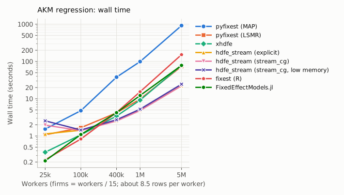
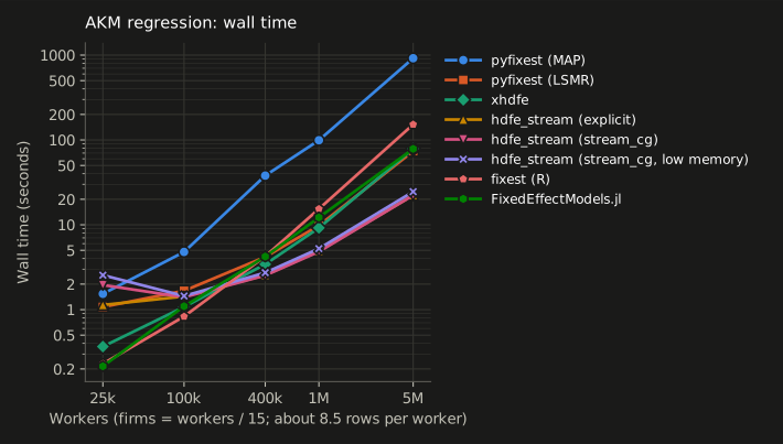
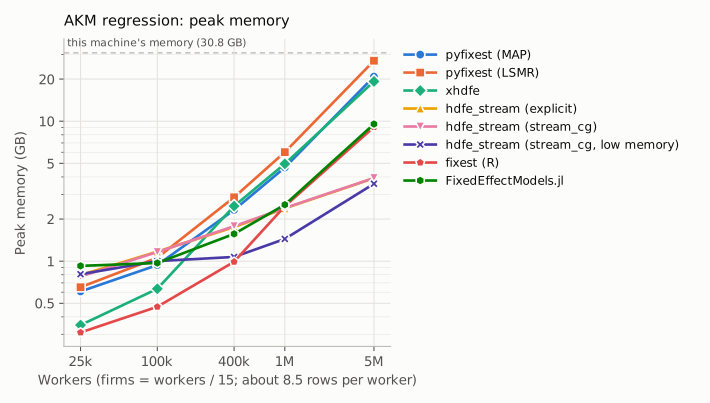
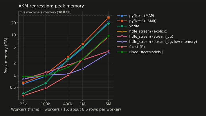
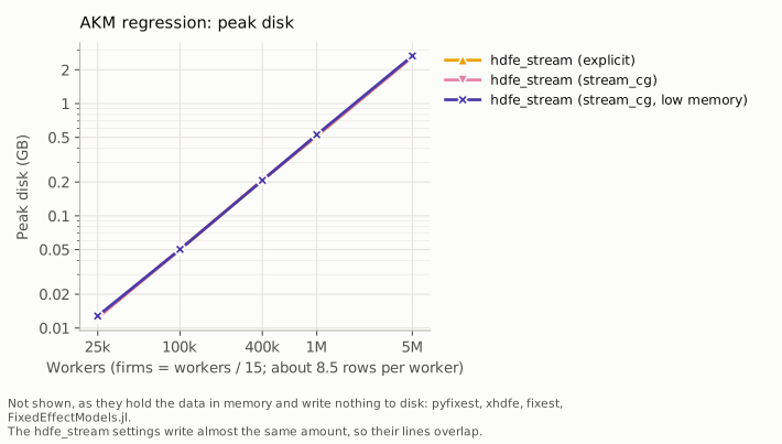
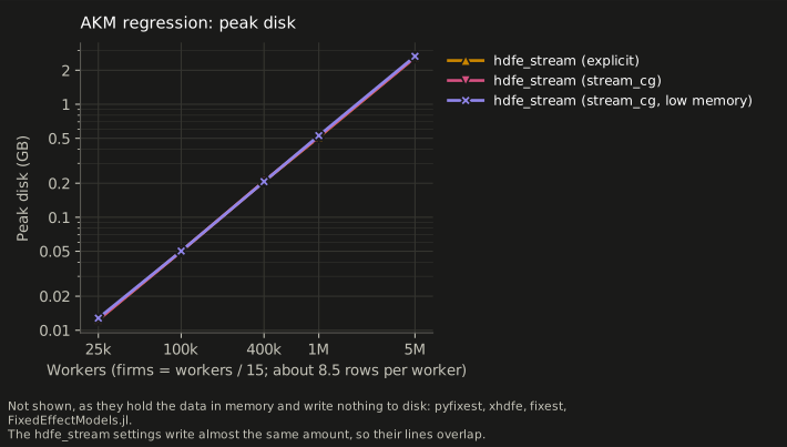
At 5 million workers:

configuration	wall time	peak memory	peak disk
pyfixest (MAP, its default)	919 s	20.8 GB	—
pyfixest (LSMR)	74 s	27.0 GB	—
xhdfe	79 s	19.3 GB	—
hdfe_stream (explicit, its default)	22 s	3.9 GB	2.6 GB
hdfe_stream (stream_cg)	22 s	3.9 GB	2.6 GB
hdfe_stream (stream_cg, low memory)	25 s	3.6 GB	2.7 GB

Reading the figures

Memory is the point. At 5 million workers the in-memory libraries peak at 19–27 GB: pyfixest’s LSMR run needed 27.0 GB of this machine’s 30.8 GB. hdfe_stream peaks at 3.9 GB with its defaults and 3.6 GB with the batch and bucket sizes turned down (“low memory”: rows_per_bucket=250_000, batch_rows=200_000), for about 10% more time and the same answer. What it spends instead is disk: about 61 bytes per row, 2.6 GB at 42.5 million rows, freed when the fit finishes. The in-memory libraries’ peak grows in proportion to the data. hdfe_stream’s low-memory setting grows far more slowly: 0.8 GB at 25,000 workers, 1.4 GB at a million, 3.6 GB at five million.

It is not slower for it. From 400,000 workers up, hdfe_stream is the fastest configuration measured: 2.6 s against xhdfe’s 3.4 s there, and at 5 million workers 22 s against pyfixest’s 74 s (LSMR) or 919 s (MAP) and xhdfe’s 79 s. Below that xhdfe is faster, by a second or less at 100,000 workers (1.1 s against 1.4 s). With AKM panel data, reducing rows to worker-firm cells before solving more than pays for the disk traffic. The simulated panel has about 8.5 rows per worker and one cell per row, which suits this approach; a specification where the cell table is no smaller than the data, and the fixed effects are less local, may do worse.

At 100,000 workers and below, the in-memory libraries use less memory. Running any hdfe_stream fit costs about 0.8 GB, most of it importing polars, numba and scipy and starting Polars’ streaming engine and numba’s thread pools. On small data that floor dominates: at 25,000 workers xhdfe peaks at 0.35 GB and pyfixest at about 0.6 GB, and at 100,000 xhdfe still needs 0.63 GB against hdfe_stream’s 1.2 GB. By 400,000 workers hdfe_stream uses the least (1.8 GB, against 2.5 GB for xhdfe and 2.9 GB for pyfixest’s LSMR). This is the concrete version of “use pyfixest (or xhdfe) if your data fits”.

The default pyfixest demeaner is not the one to compare against. MapDemeaner (alternating projections) is 9 to 12 times slower than LsmrDemeaner from 400,000 workers up, since many worker effects are the case alternating projections struggles with. If you are comparing, compare against LSMR.

hdfe_stream’s within solver uses more memory at scale: 15.1 GB at 5 million workers, where stream_cg and explicit stay near 4 GB. Prefer those when memory is the constraint.

Trading memory for time

Same data, same solver, same answer, varying only how much is in flight at once:

python benchmarks/akm_benchmark.py --memory-sweep 1000000

8,500,353 rows, 1,000,000 worker effects

rows_per_bucket	batch_rows	wall time	peak memory	peak disk
20,000,000 (default)	2,000,000	4.9 s	2,312 MB	512 MB
1,000,000	500,000	4.9 s	1,446 MB	520 MB
250,000	200,000	5.3 s	1,313 MB	526 MB
100,000	100,000	5.7 s	1,445 MB	524 MB

Most of the saving comes from the first step down, at no cost in time; the second saves a little more for 8% more time, and below that the peak rises again. The defaults are tuned for a machine with room to spare; if memory is the binding constraint, set rows_per_bucket to something near what you can afford and leave the rest alone (with many covariates, scale batch_rows and row_group_size down too; see many covariates). rhs_block bounds the other big array (levels × variables), and max_s_gb caps the explicit reduced matrix, above which solver="auto" falls back to stream_cg by itself. Out of core describes each option.