Many covariates

The same kind of comparison as the AKM regression, holding the data fixed and varying its width: the million-worker panel (8.5 million rows, 66,665 firms) with age entered as indicators, log_earn ~ i(age_bin) | worker_id + firm_id, clustered by worker, in bins from five years wide (8 indicators) down to one month (503). hdfe_stream runs at its defaults and “sized to the design”, with bucket, batch and row-group sizes scaled down as the design widens (the rule is below). Every configuration that finished agrees with every other to within 1e-8.

python benchmarks/covariates_benchmark.py

The numbers are in benchmarks/results/covariates.csv.

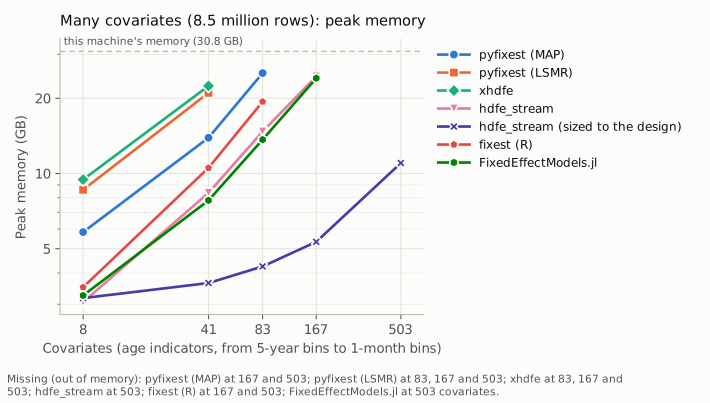
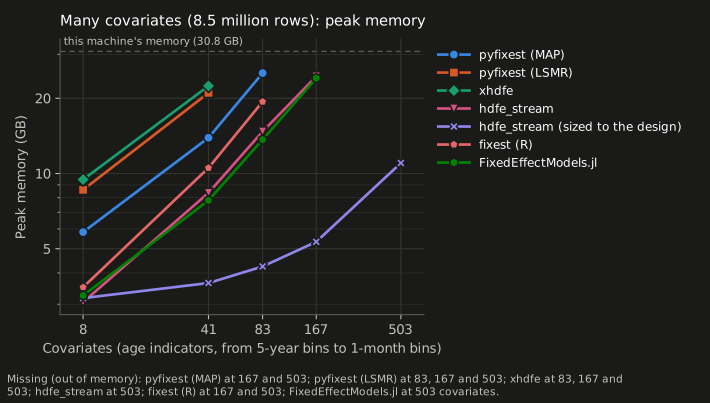
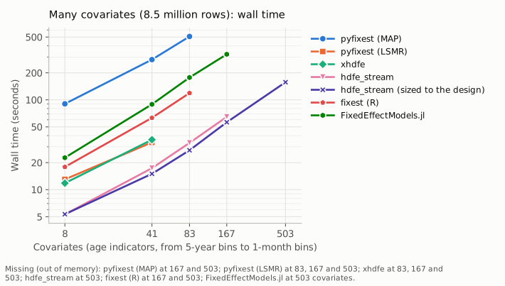
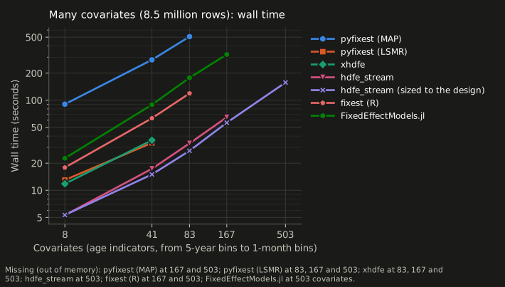
Wall time and peak memory (”—”: killed at this machine’s limit, 29.6 GB of its 30.8 GB):

covariates	pyfixest (MAP)	pyfixest (LSMR)	xhdfe	hdfe_stream	hdfe_stream, sized
8	90 s, 5.8 GB	13 s, 8.6 GB	12 s, 9.5 GB	5 s, 3.1 GB	5 s, 3.2 GB
41	280 s, 13.9 GB	34 s, 21.0 GB	36 s, 22.4 GB	17 s, 8.4 GB	15 s, 3.6 GB
83	507 s, 25.2 GB	—	—	33 s, 14.7 GB	27 s, 4.2 GB
167	—	—	—	65 s, 24.5 GB	56 s, 5.3 GB
503	—	—	—	—	157 s, 11.0 GB

Reading the figures

The in-memory libraries run out first. Their peak grows with rows × covariates. At 8.5 million rows pyfixest’s LSMR demeaner and xhdfe were out of memory at 83 indicators, and MAP, which holds the least, used 25.2 GB there and was out of memory at 167. hdfe_stream sized to the design goes from 3.2 GB at 8 indicators to 5.3 GB at 167 and 11.0 GB at 503. Part of that last figure is the memory-mapped cell table, whose pages count towards the peak although the kernel can drop them under pressure, so the memory the fit itself needs is less.

Size the batches to the design. At its defaults hdfe_stream holds a whole bucket of up to 20 million rows, with every covariate, while it sorts; that is fine for a handful of covariates and not for hundreds (24.5 GB at 167, out of memory at 503). Every step that holds rows holds all the covariates, so scale rows_per_bucket, batch_rows and row_group_size down with the width. The benchmark aims at about 1 GB of design per bucket and 250 MB per batch and row group, never above the defaults:

per_row = 8 * (k + 4)                   # k covariates, plus outcome and ids
batch = min(2_000_000, int(250e6 // per_row))
fit = feols_stream(fml, data, rows_per_bucket=min(20_000_000, int(1e9 // per_row)),
                   batch_rows=batch, row_group_size=min(500_000, batch))

Wide designs puts this together.

Time grows with the width. The cross-products cost k × k per row; they are formed chunk by chunk as BLAS matrix products. With this machine’s 16 cores the time grew about in proportion to the width from 83 indicators up, though (2.1 times from 83 to 167, 2.8 times from 167 to 503), and 503 indicators took 2½ minutes where 167 took under a minute. hdfe_stream is the fastest configuration at every width measured.

Timings are noisy where memory is tight. Each point is one run, so differences of 15% or so between configurations should not be read as meaningful. The differences between libraries above are far larger than that.

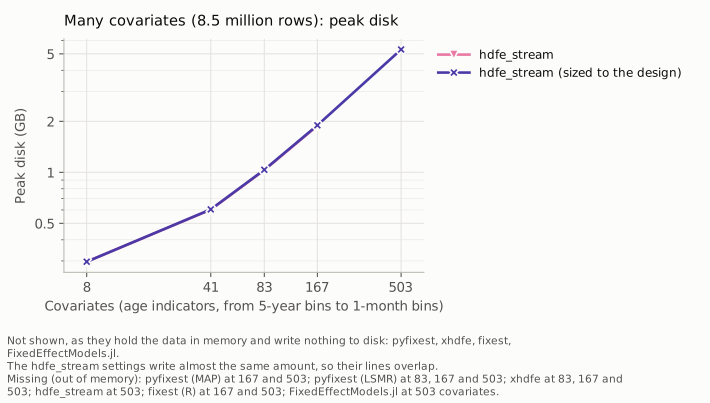
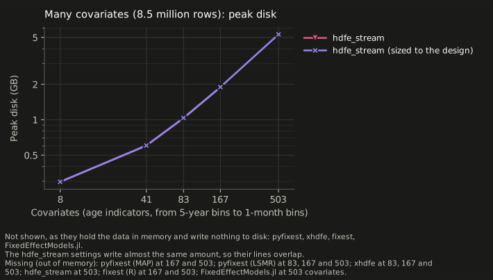
Disk grows with the width too, since the working copy of the rows carries every covariate: 0.3 GB at 8 indicators, 5.3 GB at 503.

How the design is built matters. A formula term such as i(age_bin) is carried through the partitioning as the one column it is computed from, and the indicators are built one bucket at a time. An expression that needs the whole column, possible only with the low-level interface, makes the fit build the design up front instead; see wide designs.