KSS

The whole decomposition is compared with xhdfe on its CPU backend. That means pruning, fitting, partialling out the controls, collapsing to matches, random-projection leverages and the correction, plus standard errors when asked. The model is log_earn ~ age_squared + age_cubed | worker_id + firm_id, on the same simulated panels as the regression benchmark (firms = workers / 15). Both libraries leave out a match, follow LeaveOutTwoWay’s conventions, and use 200 random-projection draws. For the standard errors each uses its own defaults: xhdfe simulates the trace term with 1,000 draws of the quadratic form, hdfe_stream with 200 Hutchinson draws (see methodological differences §5.2). At every size the two point estimates agree to within 0.3%, and from 100,000 workers up to within 0.12%, which is random-projection noise. The numbers are in benchmarks/results/kss.csv.

python benchmarks/kss_benchmark.py
python benchmarks/plot_benchmarks.py

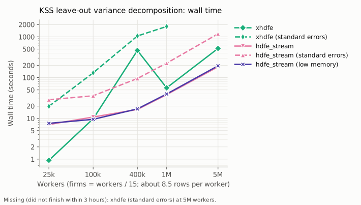
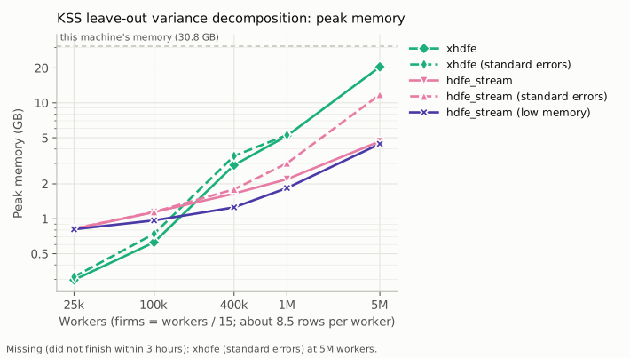
At 5 million workers (42.5 million rows):

configuration	wall time	peak memory	peak disk
xhdfe	518 s	20.4 GB	—
xhdfe, standard errors	did not finish within 3 hours (tried once; no longer run at this size)
hdfe_stream	184 s	4.7 GB	2.6 GB
hdfe_stream, standard errors	1,182 s	11.8 GB	3.2 GB

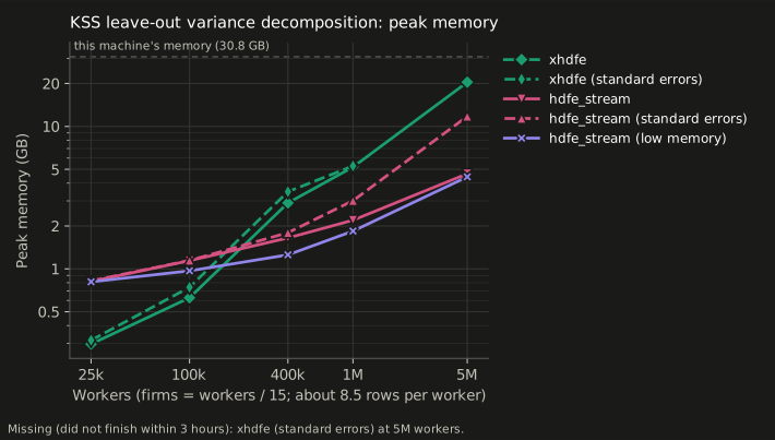
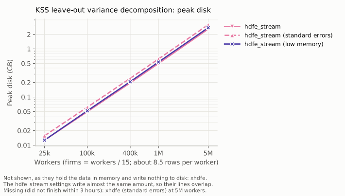
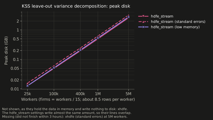
At scale, memory is the difference. At 5 million workers xhdfe’s point estimate peaks at 20.4 GB, and hdfe_stream’s at 4.7 GB, while writing 2.6 GB to disk. With standard errors hdfe_stream peaks at 11.8 GB, still a little over half of xhdfe’s point estimate alone. Both prune to exactly the same sample at every size, and at 5 million workers their estimates agree to within 0.01%.

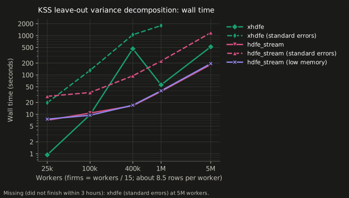
Standard errors are where the time goes. From 100,000 workers up, hdfe_stream’s are 3.7 to 11 times faster than xhdfe’s: 225 s against 1,794 s at a million workers. At 5 million, xhdfe’s did not finish in the three hours allowed (the benchmark does not run it above a million workers any more, so a rerun does not spend three hours showing that again) and hdfe_stream’s took 20 minutes. The two estimate the trace term differently (methodological differences §5.2); xhdfe’s default is 1,000 simulated draws of the full quadratic form.

Small panels favor xhdfe. At 25,000 workers its point estimate takes 0.9 s and 0.30 GB, against hdfe_stream’s 7.1 s and 0.8 GB, and at 100,000 the two are level (9.8 s against 10.8 s). hdfe_stream pays fixed costs a small panel cannot amortize: importing its dependencies, and two fits (the regression and the collapsed match-level one), each with its own passes over the data.

xhdfe’s 400,000-worker point is its solver routing, not noise. By default it factors the firm system directly up to 50,000 firms and iterates above that. At 400,000 workers (26,661 firms) its point estimate takes 462 s, against 56 s at a million workers. The factorization accounts for most of it: in an earlier check on a smaller machine, a run with 10 draws instead of 200 took nearly as long. At a million workers (66,665 firms) it iterates, and its point estimate takes 56 s, against hdfe_stream’s 38 s.

The low-memory setting helps less here than for the regression. rows_per_bucket and batch_rows shrink the fits: 1.8 GB against 2.2 GB at a million workers, and 4.4 GB against 4.7 GB at 5 million, so most of the peak is set by something those settings do not control.

scratch_mb

scratch_mb (default 32) is leave-out estimation’s own memory knob, because its passes hold about a dozen float64 columns per row of the chunk. It shrinks the chunk below batch_rows to stay inside the budget, and it changes memory only: every random vector involved is keyed on the absolute row ordinal, so the answer is bit-identical at any setting. On a 1.3M-row panel with standard errors, leaving out an observation:

scratch_mb	wall time	peak above the fit
16	61 s	46 MB
32 (default)	30 s	67 MB
128	24 s	188 MB
512	20 s	669 MB

The default sits at the knee. The point estimate on its own stays inside the peak the fit has already reached, so it adds nothing measurable.